How YouTube Finds Your Next Video in Milliseconds
A deep dive into two-tower retrieval, in-batch negatives, and the tricks that make it work
This is Part 4 of the RecSys for MLEs series. We’re now in the heart of the modern recommendation stack—the retrieval layer.
In my previous posts in this series, we discussed the high-level architecture of recommendation systems, the history of recommendation systems and the fundamentals of Recsys . But theory only goes so far; nothing truly clicks until you see the implementation and understand the engineering trade-offs required at scale. Today, we’re diving into the dominant architecture powering candidate generation at YouTube, Pinterest, Airbnb, and virtually every large-scale system: The Two-Tower Model.
What We’ll Cover Today:
The Scale Problem: Why the “brute force” approach to scoring fails at the billion-item scale.
Architectural Decoupling: How the Two-Tower design allows for sub-millisecond retrieval through offline precomputation.
YouTube’s Canonical Design: Learning from the features that defined the standard, including watch history and the “Example Age” trick.
Training at Scale: Implementing In-Batch Negatives to turn a massive classification problem into a tractable one.
Debiasing & Optimization: Using LogQ Correction to fix popularity bias and Hard Negative Mining to improve model discrimination.
Hands-on Implementation: A complete PyTorch (Code from Scratch) walkthrough using the MovieLens-1M dataset.
By the end of this post, you’ll understand why two-tower models are the “gold standard” for scale and how to build one that actually generalizes to real-world users.
The Scale Problem
Before diving into architecture, let’s understand the problem we’re solving. Imagine you’re building YouTube’s recommendation system.
You have:
2 billion+ videos in your catalog
2 billion+ users visiting daily
~100 milliseconds to return recommendations when someone opens the app
The naive approach would be to score every video for every user. This requires 2 billion forward passes per request because you will need to test each item for one user. At 1 ms per inference, that’s 23 days of compute. Per request. Obviously impossible. Would you wait for 23 days to see the recommendations?
This is the fundamental issue with retrieval: you need to find the best items, but you can’t afford to look at all of them.
Idea: The Two-Stage Solution
So the main idea behind a two tower system is simple. Why to do everything in one step? We can effectively break the problem into to parts here:
Retrieval: Just find me the best candidates to score. It doesn’t need to be perfect — it just needs to not miss good candidates.
Ranking: Score these candidates.
This division of labor is what makes billion-scale recommendations tractable.
But Why there are Two Towers here?
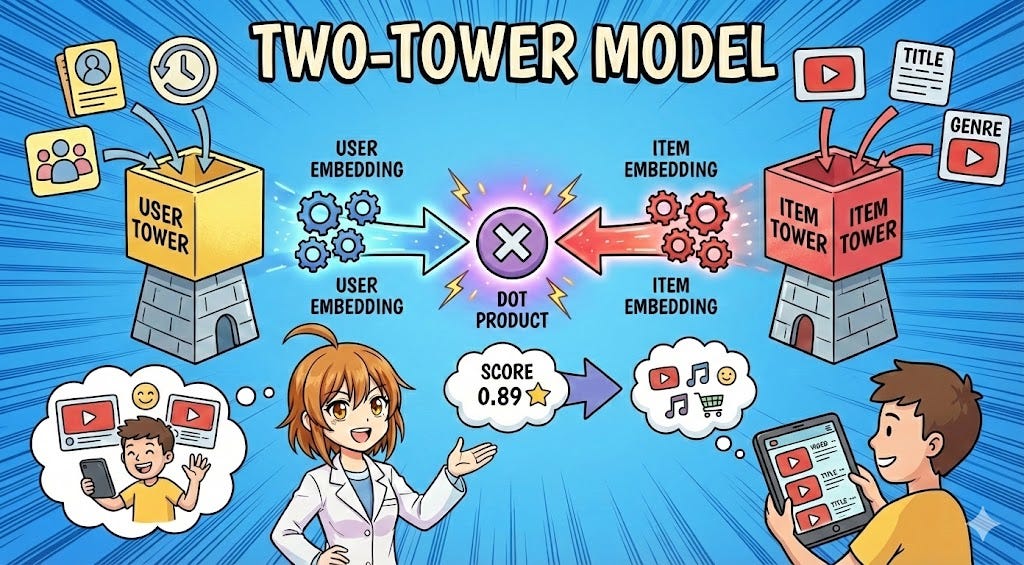
Two-tower models solve the retrieval speed problem with one clever insight: if user and item representations are independent, we can precompute item embeddings offline.
The key constraint is that the two towers never interact until the final dot product. No cross-features, no attention between user and item, no shared layers. This seems limiting, but it’s exactly what enables the incredible scale achieved by such systems:
Offline precomputation: Compute all item embeddings once, store in an index
Fast online serving: At request time, only compute the user embedding (single forward pass)
Approximate nearest neighbor search: Use FAISS/ScaNN to find top-K similar items in milliseconds
The DSSM Origins
I always love to look at the history it took us to reach the current state and the Two-tower architectures trace back to Microsoft’s Deep Structured Semantic Model (DSSM), published in 2013 for web search.
The problem DSSM solved → given a search query “machine learning tutorials,” how do you find relevant documents from billions of web pages? Traditional approaches relied on keyword matching (BM25), but this misses semantic similarity — a document about “ML courses” is relevant even without exact word overlap.
DSSM’s insight was to embed queries and documents into the same vector space, where semantic similarity corresponds to geometric proximity.
Now, the same principle applies directly to recommendations:
Query → User (what they want)
Document → Item (what we’re recommending)
Relevance → Engagement probability
DSSM showed this could work at scale. And YouTube, Pinterest, and others adapted it for recommendations. But the main thing to understand is that we are standing on the shoulder of giants.
YouTube’s Deep Neural Network (2016)
Google’s “Deep Neural Networks for YouTube Recommendations“ paper remains the canonical reference for production two-tower systems. It’s worth understanding in detail because the lessons might transfer directly to any retrieval system you’ll build.


