
The 3-Stage Funnel Behind Every Modern Recommender System
Two-Tower models, vector databases, cross-encoders—and how they work together at scale

You’re the lead engineer at YouTube.
A user just opened the app.
You have 200 milliseconds to return your recommendations to the user.
In that time, you need to scan 5 billion videos and surface the 10 they want to watch right now. Not 10 random videos. Not 10 popular videos. The perfect 10 for this specific user at this specific moment.
Miss the window? They close the app.
Show irrelevant content? They close the app.
Recommend something they watched yesterday? They close the app.
Here’s some envelope math: if your model takes just 10 milliseconds to score a single video, scoring the full catalog would take 500 days. And you have less than a second.
This is the brutal reality of production recommender systems. Training a state-of-the-art model is only 20% of the work. The other 80% is figuring out how to actually serve it.
In Post 1, we covered the fundamental techniques of recsys systems. In Post 2, we traced the history from collaborative filtering to deep learning. This post is about what happens after you have a model—how Google, Netflix, and Spotify serve recommendations to billions of users without melting their servers or losing their audience?
The answer isn’t a single clever algorithm. It’s a system design principle: don’t solve the whole problem at once.
The architecture behind every massive recommender system is in essence just a pipeline of filters. It starts with a wide net and ends with sort of a microscope.
Instead of running your smartest model on every item, you split the problem into three stages—each with a different job and a different mathematical objective.
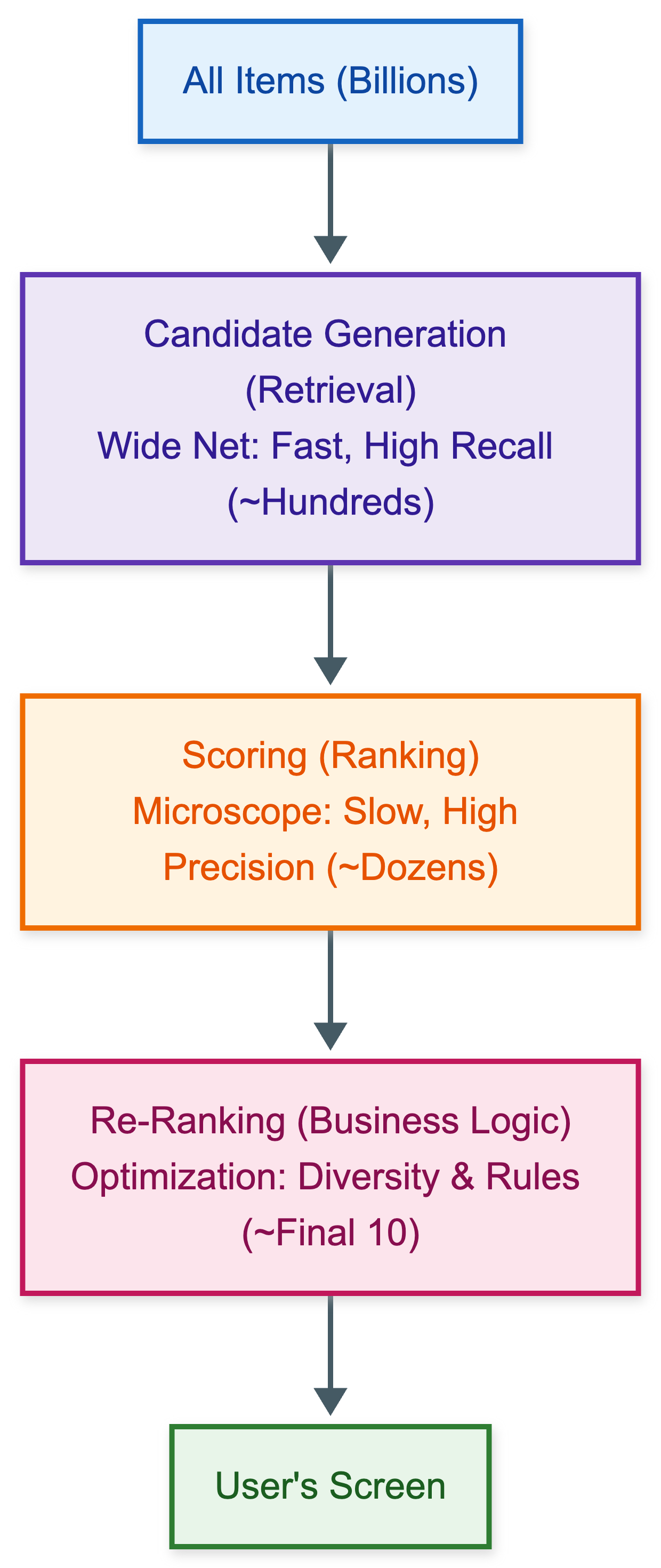
Stage 1 is Candidate Generation (The “Retrieval” Layer). The goal here is high recall—we need to go from billions of items down to just a few hundred fast. The idea is simple: we don’t care if we include some bad items, as long as we catch all or most of the relevant ones. To achieve this scale, we rely on fast, “approximate” algorithms like Vector Databases, Quantization and Two-Tower Models which we are going to discuss in this post.
Stage 2 is Scoring (The “Ranking” Layer). Once we have whittled the list down to a few hundred, we switch our goal to high precision. Because the list is small, we can now afford to spend expensive compute power to analyze the items deeply. This is where we deploy our heavy Deep Learning models, such as Cross-Encoders, Transformers, MMOE Models to determine the exact order of preference.
Stage 3 is Re-Ranking (The “Business” Layer). We now have the top dozen items, but we need to optimize for policy. The model might love these 10 items, but are they actually good for the product? This stage uses rule-based logic to handle diversity, fairness, and removing clickbait.
Stage 1: The Retrieval Layer (Candidate Generation)
The goal of this layer is fast recall. Out of billions of items, grab a few hundred that are relevant to the user.
Note that perfect ordering doesn’t matter here. It’s fine if the 5th best item lands at position 10, or if some irrelevant items slip through. What’s not fine is missing the best items entirely—because if retrieval misses it, ranking never sees it and our models don’t get to learn about good items at all.
To achieve this we rely on a specific neural architecture that has become the industry standard for this task: the Two-Tower Model (also known as a Bi-Encoder or a Dual Encoder).
The Two-Tower Architecture
We briefly touched on this in Post 2, but let’s look at it again a bit deeper this time.
A Two-Tower model basically consists of two independent deep neural networks:
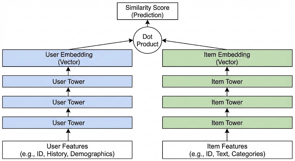
The User Tower (Query Tower): This network takes everything we know about the user right now—their watch history, their current location, the time of day, their declared interests—and passes these through several layers of a Deep Neural Network (DNN). The output is a single, dense vector (embedding), usually of a fixed size like 128 or 256 dimensions. Let’s call this vector
uThe Item Tower (Candidate Tower): This network takes everything we know about an item—its title, description, tags, video thumbnails, audio transcript—and processes it through its own DNN. The output is also a single dense vector in the exact same mathematical space as the user vector. Let’s call this vector
v.
How do they interact?
During training, both towers learn to place users and items they like close together in vector space. We measure “closeness” with a dot product (or cosine similarity).
Score = u . v
If the score is high, the vectors point in similar directions, and it’s a good match.
Training (InfoNCE Loss)
How do we actually train this? We want the dot product
to be high for items the user watched, and low for items they didn’t.
Standard classification is inefficient here because of the massive class imbalance (1 positive vs 5 billion negatives). Instead, we use Softmax Cross-Entropy with In-Batch Negatives (often called InfoNCE loss).
For a batch of size B we treat the i-th user-item pair as positive, and every other item in the batch as a negative for that user.
Where tau is a temperature hyperparameter which can be tuned. This allows us to train efficiently on massive datasets without explicitly mining billions of negative samples.
The “Hack”: Decouple these Towers
So, we have trained our two tower model. But if we ran both towers in real-time for every item, we’d gain nothing—still billions of forward passes.
