Vector Search at Scale: The Production Engineer's Guide

IVF partitions space. PQ compresses memory. Together they make 100M vector search actually possible

This is Part 5 of the RecSys for MLEs series. We’re now taking a brief foray into a vital production infra → The vector databases.

---

In my previous posts in this series, we talked about the topics below. Do take a look at them:

1. High-level architecture of recommendation systems,

2. the history of recommendation systems,

3. the fundamentals of Recsys, and

4. two tower retrieval.

---

Yesterday, a colleague asked me about Product Quantization. I tried to explain it and twenty minutes later, we were both completely lost.

It started simply enough: “What is PQ Quantization?” Then we went straight to IVFPQ.

I started explaining—IVF partitions the space, PQ compresses the vectors, you combine them for speed and memory efficiency. Easy, right?

“Okay, but what’s IVF doing exactly?”

I started explaining Voronoi cells and centroids. He asked how that connects to PQ.

At some point, we both realized neither of us could clearly articulate how all these pieces fit together. I knew IVF-PQ worked as I had used FAISS dozens of times. But explaining it from scratch was pretty hard.

So I went back and actually figured it out.

This is the explanation I wish I’d given him yesterday.

So, get a Coffee and let’s go!!!

Here’s what we’ll cover in this detailed breakdown of Vector Search:

1. Brute Force — Doesn’t Scale

2. IVF (Inverted File Index) — Partitioning space for sub-linear search

3. Product Quantization (PQ) — Compressing vectors by 64x

4. IVF-PQ Combined — Best of both worlds

5. Metadata Filtering — Combining semantic search with structured filters

6. Vector Databases — FAISS, Milvus, Pinecone, and friends

7. Benchmarking — Measuring what matters

8. Best Practices — Configuration, tuning, and pitfalls

9. Conclusion — Putting it all together

This is Part 5 of the RecSys for MLEs series. We’re now taking a brief foray into a vital production infra → The vector databases.

In my previous posts in this series, we talked about the topics below. Do take a look at them:

1. High-level architecture of recommendation systems,

2. the history of recommendation systems,

3. the fundamentals of Recsys, and

4. two tower retrieval.

1. The Problem: Brute Force Doesn’t Scale

First, let’s understand why naive nearest neighbor search fails at scale.

import numpy as np
import time

def brute_force_search(query, database, k=10):
    """Find k nearest neighbors by computing all distances."""
    distances = np.sum((database - query) ** 2, axis=1)
    return np.argsort(distances)[:k]

# Simulate different scales
for n in [10_000, 100_000, 1_000_000, 10_000_000]:
    d = 128
    database = np.random.randn(n, d).astype(np.float32)
    query = np.random.randn(d).astype(np.float32)

    start = time.time()
    indices = brute_force_search(query, database)
    elapsed = time.time() - start

    memory_gb = (n * d * 4) / (1024**3)
    print(f"n={n:>10,}: {elapsed*1000:>8.1f}ms, memory={memory_gb:.2f}GB")

Output:

n =     10,000:     25.2ms, memory=0.00GB
n =    100,000:     36.7ms, memory=0.05GB
n =  1,000,000:    391.3ms, memory=0.48GB
n = 10,000,000:   4536.0ms, memory=4.77GB

The problem is O(n × d) — linear in both dataset size and dimension. At 1 billion vectors, you’re looking at 453 seconds per query — which is totally unacceptable! Also, the size of the dataset is going to be pretty high so you couldn’t really fit it into the memory.

So, we will need techniques that provide:

1. Sub-linear search time — Don’t look at every vector.

2. Memory compression — Store vectors more efficiently.

3. Approximate results — Trade some accuracy for massive speedups.

---

2. IVF: Inverted File Index

The first key insight that we will go into is → don’t search everything. Instead, partition the space into regions and only search the relevant ones.

We can do this using IVF, which uses k-means clustering to divide the vector space into nlist partitions (also called Voronoi cells). Each partition is defined by a centroid, and thereby every database vector is assigned to its nearest centroid.

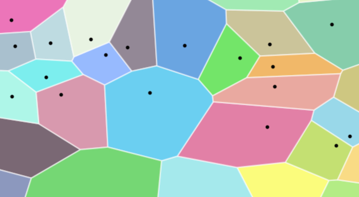
Here is how the whole IVF process works →

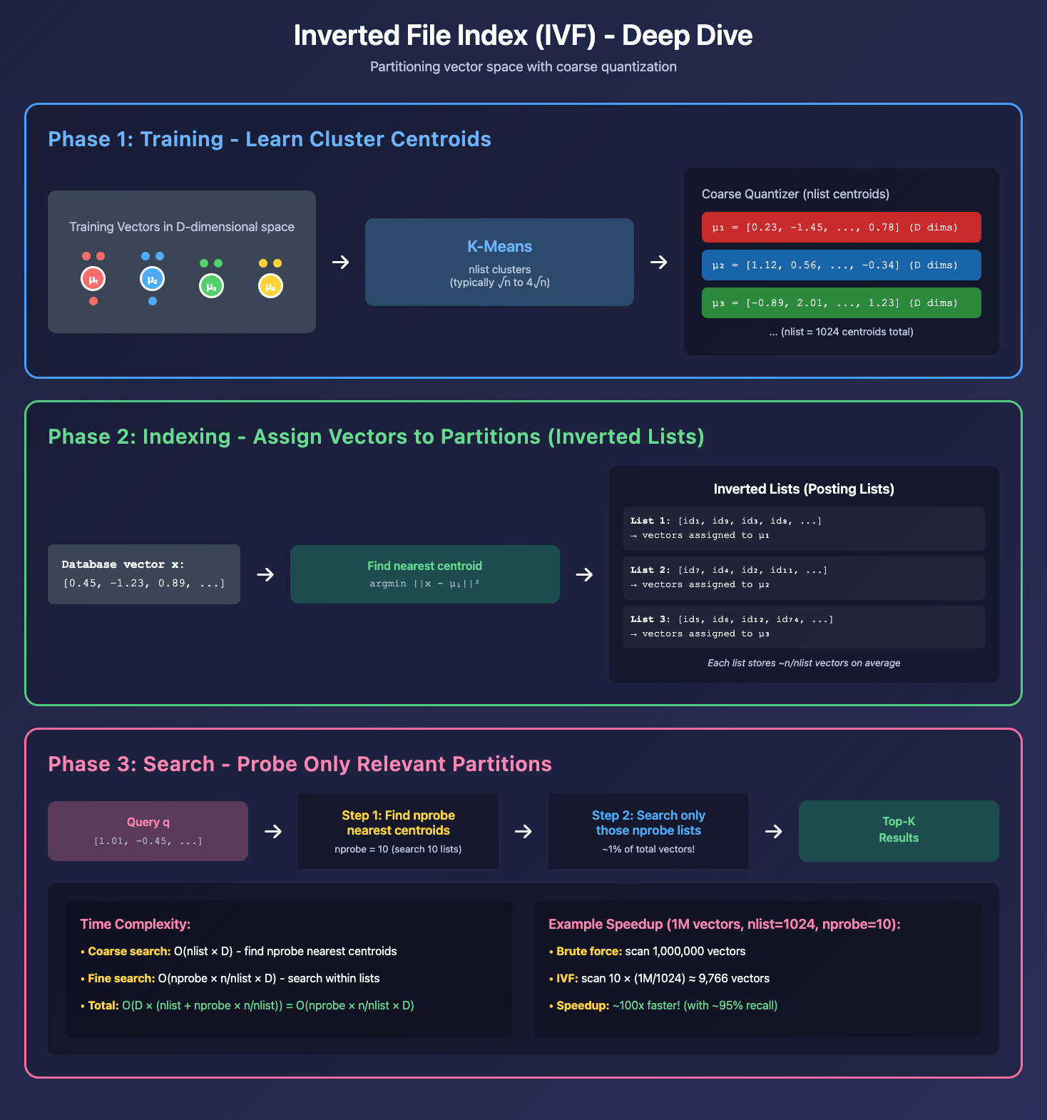
We have three distinct phases here. For better understanding, let’s think of this with some numbers. Assume that we have a total of 1M embeddings that we want to index.

A. Training Phase:

We begin by applying the k-means algorithm to a representative sample of our embedding dataset. This process identifies nlist centroids, which define the boundaries of our Voronoi cells.

• Example: If we set nlist = 1024, the vector space is partitioned into 1024 distinct clusters.

B. Indexing Phase:

Once we have nlist cluster centroids, we effectively index our entire dataset using them. Particularly, for each database vector, we find its nearest centroid and store the vector in that centroid’s “inverted list”. So we will have a total of nlist lists.

• Example: In our case, this will come out to be 1024 lists. Each list will have on average 1M/1024 points → 976 points.

C. Search Phase:

Now, rather than performing an exhaustive (brute-force) search across all 1M points, we use the nprobe parameter to limit our scope.

1. Centroid Selection: When a query vector arrives, we first calculate its distance to all nlist centroids to find the nprobe closest ones. If nprobe = 10 we will select the 10 closest centroids.

2. Localized Search: Now, rather than searching across all vectors, we will only search the vectors contained within the 10 specific Voronoi cells. So, instead of 1,000,000 comparisons, we perform only ~9,760 comparisons now, reducing the computational load by over 99%.

The idea here is that rather than searching in all cells, we search in the top 10 cells closest to the query vector.

Why does it improve speed?

• Brute force: We needed to search all n vectors → O(n × d)

• IVF: We just searched nprobe × (n/nlist) vectors → O(nprobe × n/nlist × d)

• Speedup Factor: nlist/nprobe

For 1M vectors with nlist=1024 and nprobe=10:

• Brute force: 1,000,000 distance computations

• IVF: 10 × (1M/1024) ≈ 9,766 distance computations

• Speedup: ~100x!

Now, here is how we can implement this using FAISS.

import faiss
import numpy as np
import time

# Simulate different scales
for n in [100_000, 1_000_000, 10_000_000]:
    d = 128
    database = np.random.randn(n, d).astype(np.float32)
    query =  np.random.random((1, d)).astype('float32')

    # Number of Voronoi cells
    nlist = 1024                  
    # The coarse quantizer (how we find centroids)
    quantizer = faiss.IndexFlatL2(d)  
    index = faiss.IndexIVFFlat(quantizer, d, nlist)
    
    # 3. Train & Add
    # Training on the whole set is slow. 
    # FAISS usually trains on a subset (e.g., 10k points).
    index.train(database[:100000])
    
    index.add(database)
    
    start = time.time()
    indices = index.search(x=query,k=10)
    elapsed = time.time() - start
    
    print(f"n={n:>10,}: {elapsed*1000:>8.1f}ms")

Output:

n=   100,000:      0.2ms
n= 1,000,000:      0.4ms
n=10,000,000:      1.3ms

This is all good and great, but as you know, there is no free lunch. The Trade-off here is between Recall vs Speed.

While we have increased speed, if the true nearest neighbor is in a partition we didn’t probe, we’ll miss it.

Also note that IVF doesn’t reduce memory. It just reduces the search space—we are still storing full float32 vectors. And that’s where PQ comes in.

---

3. Product Quantization (PQ): Vector Compression

IVF speeds up search but doesn’t help with memory. At 1 billion 128-dimensional vectors in float32, you need 512 GB of RAM. Product Quantization effectively compresses this to 8 GB—a 64x reduction. But How?

It is a Divide and Quantize paradigm.

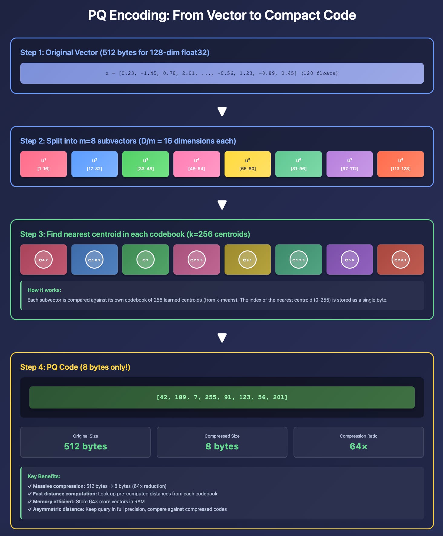
PQ works by:

1. Splitting each vector into m subvectors

2. Clustering each subspace independently with k centroids

3. Encoding each subvector as the ID of its nearest centroid

Let’s look at an example through a 128-dimensional vector with m=8 subvectors and k=256 centroids:

Original vector (512 bytes):

x = [0.23, -1.45, 0.78, ..., 0.45]  # 128 floats × 4 bytes = 512 bytes

Split into 8 subvectors (16 dims each):

u¹ = [0.23, -1.45, ..., 0.89]   # dims 1-16
u² = [1.12, 0.34, ..., -0.56]   # dims 17-32
...
u⁸ = [-0.12, 0.67, ..., 0.45]  # dims 113-128

Find the nearest centroid in each codebook:

u¹ → codebook 1 → nearest centroid: index 42
u² → codebook 2 → nearest centroid: index 189
...
u⁸ → codebook 8 → nearest centroid: index 201

Final PQ code (8 bytes!):

pq_code = [42, 189, 7, 255, 91, 123, 56, 201]  # 8 uint8 values

Compression: 512 bytes → 8 bytes = 64x!

Till now, we talked about the codebook in a handwavy way, but here is the whole implementation on how PQ works.