From Candidates to Clicks: The Engineering Anatomy of Ranking

How modern recommendation systems go from 1,000 candidates to the one item you actually tap

Mar 14, 2026

∙ Paid

This is Part 6 of the RecSys for MLEs series. We're now in the final mile: the Ranking layer.In my previous posts in this series, we talked about the topics below. Do take a look at them:

A new engineer on our team once asked: “Why can’t we just sort by the Two-Tower scores? We already have them?”
It’s a deceptively simple question — the kind that sounds naive until you realize most experienced engineers can’t fully answer it either. The Two-Tower model is blind by design. At query time, it never sees a specific user and a specific item in the same room. The ranking model does. And that one architectural decision cascades into an entirely different class of problem.
That’s what this piece is about.

Here's what we'll cover in this detailed breakdown of Ranking:

The Ranking Problem → Why 1,000 candidates still requires a completely different model
The Feature Space → Dense, sparse, and cross features that power ranking
The Pre-Neural Era → Logistic Regression and GBDTs: why they dominated for a decade
Wide & Deep → Google's 2016 paper that changed everything
Deep & Cross Network (DCN v2) → Automatic feature crossing at scale
DLRM → Meta's production architecture powering Facebook and Instagram
Multi-Task Ranking → Why optimizing for one signal is always wrong
The Future → Lets have generative rankers
Best Practices → Configuration, trade-offs, and pitfalls

1. The Ranking Problem

Before we even start, let's be precise about what we're solving.

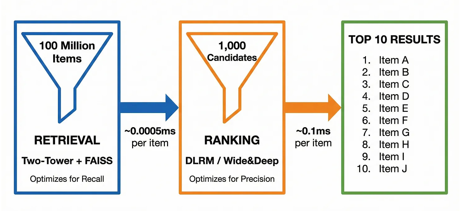
After retrieval (Two-Tower + FAISS), you have somewhere between 100 and 2,000 candidates. These are items that are semantically relevant to the user. Now you need to sort them. And sorting them badly is expensive → in ad systems, a 1% improvement in ranking quality can mean tens of millions of dollars(certainly billions for Meta). On a social feed, it's the difference between a user opening the app or deleting it and an opportunity loss forever.

The key insight is this: retrieval optimizes for recall; ranking optimizes for precision.

The entire two-stage architecture comes down to a simple budget constraint. Retrieval has to score roughly 100 million items in under 50ms — that’s 0.0000005ms per item, which is why we use approximate nearest neighbor search (FAISS) and willingly accept false positives assuming that Ranking will clean them up.

Ranking, by contrast, only sees ~1,000 survivors and has a 100ms budget — 0.1ms per item. Run the math and that’s a 200,000x larger per-item budget.

This budget difference is why ranking models look nothing like retrieval models. We can use:

Dense cross-attention over all feature pairs
Deep neural networks with hundreds of millions of parameters
Expensive feature crosses and second-order interactions
Rich user history features (last 100 interactions)

None of this is possible at retrieval scale.

2. The Feature Space

Before we even look at the models, we need to understand the features we can use in such systems. Ranking models consume a mix of three feature types, and getting this right is half the battle.

A. Dense Features (Continuous)

Dense features are your traditional ML inputs — numbers and low-cardinality categories you can encode directly:

User features — age, account tenure, average session length. Static signals about who the user is.
Item features — average CTR, content age, creator follower count. Signals about the item’s quality and reach.
Context features — hour of day, day of week, device type. The when and where of the request. Low-cardinality enough to one-hot encode or pass as-is.
Interaction features — user-category affinity, user-creator affinity, user’s recent CTR. These are the most valuable: they describe the relationship between this user and this type of content, not just each in isolation.

The last group is worth calling out. Pure user features and pure item features are static — they don’t change based on who’s seeing what. Interaction features do. That’s what makes them disproportionately predictive.

B. Sparse Features (High-Cardinality IDs)

This is where ranking models diverge sharply from traditional ML. You have features like user_id (500M unique values), item_id (1B unique values), creator_id (50M values). You can't one-hot encode these.

The solution? Embedding lookup tables.

import torch
import torch.nn as nn

# Each sparse feature gets its own embedding table
embedding_tables = {
    "user_id":    nn.Embedding(num_embeddings=500_000_000, embedding_dim=64),
    "item_id":    nn.Embedding(num_embeddings=1_000_000_000, embedding_dim=64),
    "creator_id": nn.Embedding(num_embeddings=50_000_000, embedding_dim=32),
    "category_id":nn.Embedding(num_embeddings=500, embedding_dim=16),
}

# At inference time: just look up the embedding vector for this user/item pair
user_embedding   = embedding_tables["user_id"](torch.tensor([user_id]))  # shape: [1, 64]
item_embedding   = embedding_tables["item_id"](torch.tensor([item_id]))  # shape: [1, 64]

In practice, these embedding tables are the largest part of the model -- often hundreds of GB. This is why ranking models are memory-bound, not compute-bound.

C. Cross Features

Some signals are only meaningful in combination. A user who usually watches cooking videos at 6pm might click on cooking content at 6pm but not at 2am. The feature hour_of_day=18 AND category=cooking is a cross feature.

# Manual cross feature (the old way)
user_category_hour = f"{user_top_category}_{hour_of_day_bucket}"
# e.g., "cooking_evening" -> one-hot encoded

# Neural approach: learn the crosses automatically (we'll see this with DCN)

Historically, feature engineering consumed 70% of an ML team's time. Deep learning's main promise was automating this. But as we'll see, the truth is nuanced.

3. The Pre-Neural Era: Why It Still Matters

Logistic Regression → The Original Ranker

For nearly a decade (2005-2015), the dominant ranking model at companies like Google, Yahoo, and early Facebook was Logistic Regression and honestly it still is in a lot of model stages.

You represent each (user, item, context) tuple as a sparse binary vector → one-hot encoded features → and learn a weight for each. Click prediction becomes:

P(click) = sigmoid(w1*user_london + w2*item_sports + w3*evening + ...)

import numpy as np
from sklearn.linear_model import LogisticRegression
from sklearn.preprocessing import OneHotEncoder

# Simple example: 1M training examples, sparse features
# user_region (50 values), item_category (100 values), hour_bucket (6 values)

# In practice this is millions of features wide (all possible values)
X = one_hot_encode(training_data)   # shape: [1M, ~10K features]
y = training_data["clicked"]

model = LogisticRegression(solver='liblinear')
model.fit(X, y)

Why it worked:

It was Blazingly fast. Train in minutes, can be served in microseconds.
Perfectly interpretable. The weight for "user in London" tells you exactly how much being in London affects CTR.
Scales linearly with data.

Why it doesn’t work:
The model is linear. It cannot learn that "Sports + Evening + Mobile" together drives 3x higher CTR than each feature alone. To capture this, engineers had to manually create cross features:

# "Feature Engineering Hell" -- an actual practice at early Facebook/Google

cross_features = []
for f1 in dense_features:
    for f2 in dense_features:
        cross_features.append(f"{f1}_AND_{f2}")   # O(n^2) feature explosion

# At 10,000 base features: 100,000,000 potential cross features
# Most are useless. Figuring out which ones aren't -> that's the job.

At Yahoo, teams had dedicated "feature engineers" whose entire job was designing these cross features. This didn't scale and it was a headache to mantain and have these many complex data pipelines comprising of feature engineering and feature selection.

GBDTs → The Kaggle King

Gradient Boosted Decision Trees (XGBoost, LightGBM) solved the interaction problem somewhat elegantly: each tree learns a decision rule over a combination of features. You don't need to specify sports_AND_evening manually → the tree discovers it.

import lightgbm as lgb
import pandas as pd

# Features are now dense numerical values, not one-hot encodings
X_train = pd.DataFrame({
    "user_age": user_ages,
    "user_avg_ctr": user_ctrs,
    "item_category_id": item_categories,   # LightGBM handles categoricals natively
    "hour_of_day": hours,
    "item_age_hours": item_ages,
})

y_train = clicks

dtrain = lgb.Dataset(X_train, label=y_train)

params = {
    "objective": "binary",
    "metric": "auc",
    "num_leaves": 127,
    "learning_rate": 0.05,
    "feature_fraction": 0.9,
}

model = lgb.train(params, dtrain, num_boost_round=500)

# A single tree's decision path might look like:
# if item_category == "sports" AND hour_of_day > 17 AND user_age < 35: CTR += 0.03

GBDTs dominated leaderboards for years, and they still power ranking at many companies as a baseline or for feature selection.

Where they struggle:

High-cardinality sparse features: You cannot feed 500M unique User IDs into LightGBM.
Online learning: Updating a GBDT incrementally is hard. Neural networks handle streaming updates gracefully.
Multi-modal features: Raw text, image embeddings, sequences → GBDT can't consume these natively.

And, this is exactly where the Wide & Deep network stepped in.

4. Wide & Deep: Google's Breakthrough (2016)

In 2016, the Google Play team published "Wide & Deep Learning for Recommender Systems". It's one of the most influential papers in industrial ML, and it directly addressed the LR vs. GBDT trade-off.

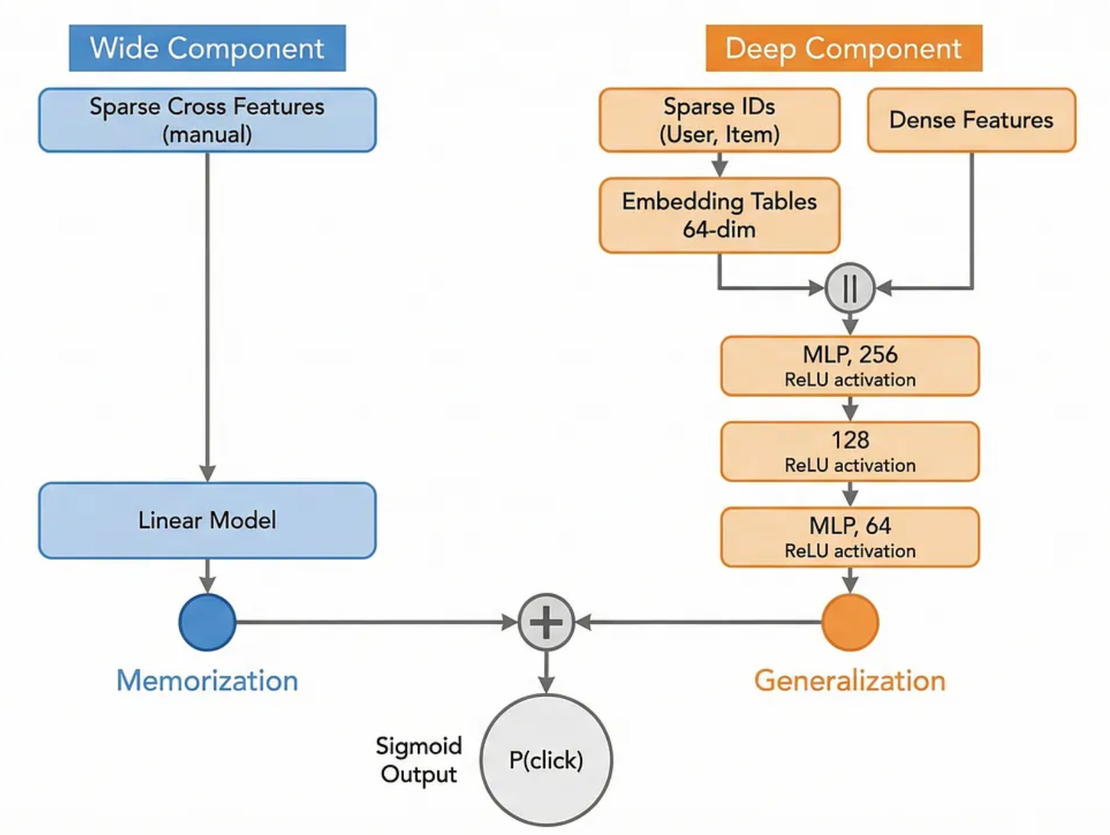
The key insight: memorization and generalization are both important, and you need a different architecture for each.

Wide component: A linear model on raw and crossed features. Good at memorizing specific patterns ("users who installed app A also install app B").
Deep component: A deep neural network on embeddings of sparse features. Good at generalizing to unseen (user, item) pairs.

You train both jointly and combine their outputs.

import torch
import torch.nn as nn

class WideAndDeep(nn.Module):
    def __init__(self,
                 num_dense_features: int,
                 sparse_feature_dims: dict,  # {feature_name: (vocab_size, embed_dim)}
                 deep_hidden_dims: list = [256, 128, 64]):
        super().__init__()

        # Wide component: linear model on dense + cross features
        self.wide = nn.Linear(num_dense_features, 1)

        # Embedding tables for sparse features
        self.embeddings = nn.ModuleDict({
            name: nn.Embedding(vocab_size, embed_dim)
            for name, (vocab_size, embed_dim) in sparse_feature_dims.items()
        })

        # Deep component: MLP on concatenated embeddings + dense features
        total_embed_dim = sum(d for _, d in sparse_feature_dims.values())
        deep_input_dim = num_dense_features + total_embed_dim

        layers = []
        in_dim = deep_input_dim
        for h_dim in deep_hidden_dims:
            layers.extend([
                nn.Linear(in_dim, h_dim),
                nn.ReLU(),
                nn.BatchNorm1d(h_dim),
                nn.Dropout(0.1),
            ])
            in_dim = h_dim
        self.deep = nn.Sequential(*layers)
        self.deep_output = nn.Linear(in_dim, 1)

    def forward(self, dense_features, sparse_features):
        # Wide path
        wide_output = self.wide(dense_features)  # [B, 1]

        # Deep path: look up embeddings for all sparse features
        embed_list = [
            self.embeddings[name](ids)
            for name, ids in sparse_features.items()
        ]
        deep_input = torch.cat([dense_features] + embed_list, dim=1)  # [B, D]
        deep_output = self.deep_output(self.deep(deep_input))          # [B, 1]

        # Joint output
        logit = wide_output + deep_output
        return torch.sigmoid(logit).squeeze(1)


# Example instantiation
model = WideAndDeep(
    num_dense_features=10,
    sparse_feature_dims={
        "user_id":    (500_000, 64),
        "item_id":    (1_000_000, 64),
        "category_id":(500, 16),
    }
)
print(f"Parameters: {sum(p.numel() for p in model.parameters()):,}")
# Output: Parameters: 96,089,804

Let's look at training this on a synthetic dataset to see it in action:

import torch
import torch.nn as nn
from torch.utils.data import DataLoader, TensorDataset
import numpy as np

# Generate synthetic ranking data
N = 100_000
torch.manual_seed(42)

dense   = torch.randn(N, 10)
user_ids = torch.randint(0, 500_000,   (N,))
item_ids = torch.randint(0, 1_000_000, (N,))
cat_ids  = torch.randint(0, 500,       (N,))

# Ground truth: users click more on items they have affinity for
# (simple synthetic rule)
labels = ((dense[:, 0] + dense[:, 2] > 0) & (cat_ids < 250)).float()

dataset = TensorDataset(dense, user_ids, item_ids, cat_ids, labels)
loader  = DataLoader(dataset, batch_size=2048, shuffle=True)

model     = WideAndDeep(10, {"user_id": (500_000,64), "item_id":(1_000_000,64), "category_id":(500,16)})
optimizer = torch.optim.Adam(model.parameters(), lr=1e-3)
criterion = nn.BCELoss()

for epoch in range(5):
    total_loss = 0
    for dense_b, uid_b, iid_b, cid_b, y_b in loader:
        pred = model(dense_b, {"user_id": uid_b, "item_id": iid_b, "category_id": cid_b})
        loss = criterion(pred, y_b)
        optimizer.zero_grad()
        loss.backward()
        optimizer.step()
        total_loss += loss.item()
    print(f"Epoch {epoch+1} | Loss: {total_loss/len(loader):.4f}")

Output:

Epoch 1 | Loss: 0.6891
Epoch 2 | Loss: 0.6204
Epoch 3 | Loss: 0.5877
Epoch 4 | Loss: 0.5701
Epoch 5 | Loss: 0.5589

Wide & Deep became the template that every major tech company adapted. YouTube, Spotify, Airbnb, and Twitter all published variants of this architecture within two years of the paper.

But there was still a manual bottleneck: the cross features in the Wide component still had to be designed by hand.

5. DCN v2: Automatic Feature Crossing

Continue reading this post for free, courtesy of Rahul Agarwal.

Or purchase a paid subscription.

MLWhiz | AI Unwrapped